Excel Formulas

If Statements

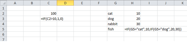
=IF(Logic test, Value if true, value if false)

For example if a cell is greater than the value 10 you can return 1, if it is not you can return 0.

Or

If the cell to the left says cat return 10, if it says dog return 20 otherwise return 30

VLookups (exact match)

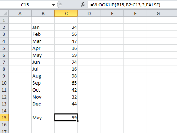
=VLOOKUP(value to lookup, area to search, column to return data from, false)

A vlookup allows you to search for a particular text or number within a column and return a value from this row, where it finds a match. The value you are searching for can either be hard coded into the formula or you can refer to a cell which has what you are trying to match.

You then enter the range that has the data to search against, and the column reference to return.

In the example below the data range is B2 to C13. This makes column B column 1, and column C column 2.

By entering a 2 in the column reference it therefore gives the answer from column C where it finds the match to "May" in column B.

By writting FALSE at the end of the formula, ensures that only exact matches are returned.

HLookups (exact match)

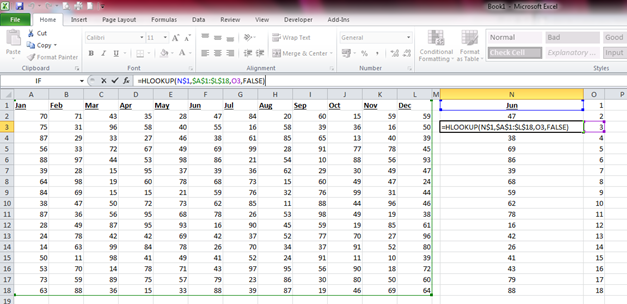
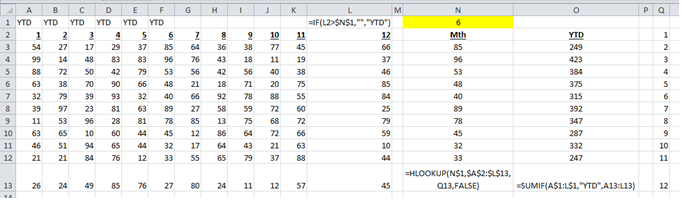
=HLOOKUP(value to lookup, area to search, row to return data from, false)

Just like a vlookup (verticle lookup) this formula for a hlookup (horizontal lookup) alows you to search across a row, and when it finds the value it is looking for, moves down the number of rows you require and returns the value from that cell.

By absoluting ($) some of the cell references, and refering to another cell for the row index number you can copy the same formula down for every row. This way for the next month you only need to change the text in cell N1 to "Jul" to change the figures in column N.

Lookup errors

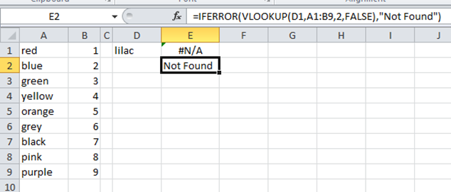
#N/A

You might get this error appear if you have a lookup where the item you are searching for is not listed.

You can fix this in two ways, the simplest is an Iferror formula where you put in the equation to use, and then what to return if it is not found. This could be text or a number or equation.

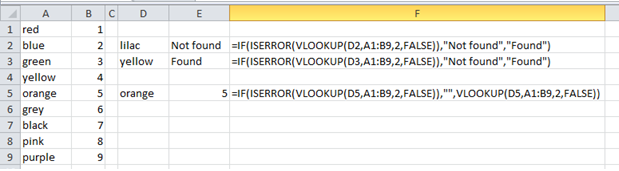
Another solution is to use if and iserror. This is a longer equation but does mean you can specify the result for a match and a non matching result.

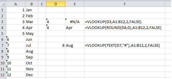
You may also get an error due to a difference in formatting.

If the table is formatted as either text or number and the lookup value is the opposite, the lookup returns an error.

You could fix this by reformatting either the data or the lookup value.

However if you do not wish to do this you can amend the lookup with a round or text formula to convert the lookup value into the same format as the data.

Right and Left Formula with a lookup

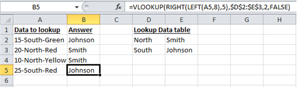
If the data you wish to lookup has other data in the cell it may be possible to use the right and left equations to only take the data you need from the cell.

This works well when the data has a defined number of digits.

The below equation takes the first 8 digits of the cell in column A, then takes the right 5 digits of that answer, and looks it up in the table.

SumIf

A sumif is great for summing a range of data where another criteria is true.

In the example below, just by changing the value in cell N1 to the new month you can change both the month figure in column N and the year to date figure in column O.

The formula in column O sums that row (columns A to L) for every column where "YTD" is found in row 1 for columns A to L.

By absoluting ($) row 1 in the formula you can drag the formula down for each row.

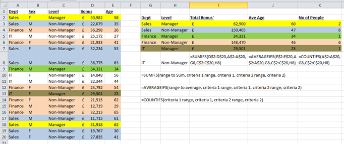
SUMIFS, AVERAGEIFS, COUNTIFS (Multiple criteria)

You can combine sum, average and count formulas with ifs so that you perform the function every time cells meet a set criteria. You can have more than 2 criteria.

In the example below the data set in columns A to E are being summed in column I, averaged in column J and counted in column K, every time the criteria in column G is matched to column A, and the criteria in column H is matched to column C.

I have highlighted the matches to make them easier to see.